

Quantitative Trading Problem Statement
Addressing the Growing Need for Data-Driven Decision-Making in Fast-Paced Financial Markets

The Math that Moves Markets
Quantitative trading is as complex as it sounds. Quants are often referred to as “the geniuses of Wall Street,” writing and maintaining code for software to execute optimal choices based on data, math, and logic.
Most have PhDs in topics covered in classes that college students typically drop out of, such as statistics, computer science, or physics.
However, for those who are new to finance or financial engineering, the real challenge is not so mathematical, but rather identifying the problem itself and aligning it with a specific trading goal:
How can we use data and mathematical models to generate consistent returns in the financial markets under specific constraints and time horizons?
This article walks you through how quantitative traders identify financial problems, translate them into mathematical models, and use those models to design strategies. You'll see how quant strategies are built as solutions to specific kinds of questions and constraints.
What are the intentions of the problem solver?
To make money, of course. But let’s be honest—everyone wants to make money. The real question is when and how do you make it consistently?
For instance:
Day traders might prioritize high-frequency, low-margin trades.
Swing traders focus on short-to-medium term reversals or trends.
Long-term investors want models that work across months or years.
Your goal shapes your math. Your intention sets the time horizon and risk tolerance, guiding the entire strategy.
What is a Quantitative Trading Problem Statement?
Now that we have our time frame, we can construct a meaningful problem statement which, when solved, yields an (ideally) optimal strategy.
The keyword here is “strategy.” Being a quant is NOT the same as being a trader. A trader directly takes positions, executes, and makes profits. Quantitative trading is about finding a strategy which informs those decisions.
A quantitative trading problem statement refers to a clear challenge or objective in the financial markets, often framed in data-driven terms. It may often include the following:
The market setup—What securities or assets are being analyzed? What data is available?
The objective—Are you trying to maximize return? Minimize risk? Find a market anomaly?
The constraints—Are there trading costs, limits on leverage, or position size caps?
How does it work?
In any trading, there is a given—buy low, sell high. In Quant Trading, the primary difference, and the reason why there’s much more potential for gains, is that it deals with maximizing the probability of achieving the maximum price difference between your sell and your buy.
The way many do this is through four common approaches:
1. Statistical Arbitrage: Exploiting price differences between related assets.
Goal: Profit from temporary price differences between related stocks
Method: Statistical analysis of price spreads
Timeframe: Minutes to Hours
Statistical arbitrage involves profiting from price differences between two or more related assets. If two stocks typically move together but temporarily diverge in price, you bet that they’ll eventually converge again.
Mathematical Model:
Where:
β = hedge ratio (number, like 0.85), which identifies how many shares of stock B to hold for each share of stock A.
You open positions when the spread deviates significantly from its mean:
Where:
μ = historical mean of the spread
σ = standard deviation of the spread which is a measure of how much prices typically vary
k= threshold constant (1 or 2) which indicates how many standard deviations the spread is away from the mean
Example: Coca-Cola trades at $60, Pepsi at $120. Normally Pepsi = 2 × Coca-Cola. Today the ratio is 2.1, so we short Pepsi and buy Coca-Cola, expecting the ratio to return to 2.0
Execution Logic: We track the difference in price between two stocks that usually move together. When that difference, or spread, becomes unusually large or small compared to its historical average, we bet that the prices will return to their usual relationship. Regression helps us hedge (reducing the risk of potential losses in one investment by making another) one asset against the other, and the standard deviation helps us detect when the spread is "far enough" from the norm to trade.
Time Frame and Market Fit: Statistical arbitrage strategies are typically used over short to medium-term horizons—ranging from intraday (minutes to hours) to a few days or weeks.
The goal is to capitalize on temporary price fluctuations before the market fixes them. Holding periods are usually short because the opportunity disappears once prices converge. This makes stat arb ideal for high-frequency trading.
2. Momentum Trading: Betting that rising stocks will keep rising (and the other way around).
Goal: Capture profits by riding short-to medium-term price trends
Method: Signal detection through trend-following indicators and price momentum
Timeframe: Multi-day to multi-week
Momentum trading is based on the idea that stocks which have performed well recently will continue to do well, and those that have done poorly will continue to fall—at least in the short term.
Mathematical Model:
Where:
Example: Tesla breaks through a key resistance level at $850 on strong volume and news of record deliveries. You buy at $855, expecting that the upward momentum will continue to push the stock higher. You ride the trend until it shows signs of reversal.
Execution Logic: We calculate how much the stock has gained or lost over a given time. If the return is significantly positive, it indicates upward momentum, so we buy expecting it to continue. If it’s significantly negative, we short the stock. The model is simple but powerful—it rides existing trends rather than trying to predict reversals.
Time Frame and Market Fit: Short to medium term. Usually days to a few weeks, though sometimes extended if the trend continues.
Momentum strategies bank on the idea that trends persist over a short-to-intermediate horizon. They don’t expect permanent gains—just that the stock will continue its recent path for a bit longer. Momentum signals weaken over time as trends fade or reverse, so holding too long can reduce gains or cause losses. This makes it ideal for swing traders or short-term trend followers.
3. Mean Reversion: Betting that prices will return to a historical average.
Goal: Profit from prices returning to their average or fair value
Method: Identify deviations from historical price averages or z-scores
Timeframe: Short to medium-term
A mean reversion strategy assumes that asset prices will tend to move back toward their historical average over time. For example, if a stock typically trades at $100 but suddenly drops to $90 without a major news reason, we might expect it to eventually bounce back to $100.
Mathematical Model:
Where:
μ = moving average of price over window of time frame n
σ = moving standard deviation over same window
z= z-score which is how unusual today's price is compared to average
Example: Apple stock usually trades around $180, but after a sharp earnings reaction, it jumps to $195. You believe this move is an overreaction and expect it to revert to its average. So you short Apple at $195, aiming to cover when it returns to its mean price of $180.
Execution Logic: The z-score shows how unusual today’s price is compared to the average of recent days. A z-score of -1 means the price is 1 standard deviation below average—potentially a buying opportunity. If the price is way above average, we consider selling. We assume extreme values don’t last forever and eventually return to normal.
Time Frame and Market Fit: Short to medium term–typically days to a few weeks, depending on the volatility.
Mean reversion strategies expect prices to return to a historical average, and that reversion often occurs within a moderate time frame. If it doesn’t, the assumption of "temporary mispricing" may be incorrect. Longer holding periods risk such changes overriding technical signals. Therefore, this strategy is best for capturing quick corrections in price.
4. Market Making: Providing liquidity by placing buy/sell orders at different price levels.
Goal: Capture bid-ask spread through providing liquidity
Method: Continuous quoting on both sides of the order book with risk controls
Timeframe: High-frequency, intraday
Market makers profit by constantly buying and selling assets at slightly different prices, known as the bid-ask spread. They place limit orders to buy at a lower price (bid) and sell at a higher price (ask), earning the difference when both orders get filled. They provide liquidity so that other traders can always find someone to trade with. Although each individual trade earns just a small profit, market makers do this thousands of times a day, relying on volume and tight risk management to stay profitable.
Market makers profit from the bid-ask spread. They buy at $99.50 and sell at $100.00, keeping the $0.50 difference.
The Problem: If you buy 1,000 shares but only sell 200, you're stuck holding 800 shares. If the price drops $1, you lose $800.
The Mathematical Solution:
Expected Profit = (Bid-Ask Spread × Volume) - (Risk Penalty × Shares Held²)
Example: You make $500 from spreads but hold 1,000 extra shares. Risk penalty might be $200, so net profit = $300.
Execution Logic: You earn a small profit every time someone hits your bid or ask. The more volume you handle, the more these small profits add up. However, if you accumulate too much of the asset (inventory risk), price movement can hurt you. So quants also build models to manage how much they hold at once. The goal is balance: make small profits frequently while staying market neutral.
Time Frame and Market Fit: Ultra-short term to intraday. Seconds to minutes. Sometimes hours.
Market making is all about high-frequency trades and capitalizing on the bid-ask spread. The goal is to make a large number of small profits throughout the day. Holding positions for longer than necessary introduces inventory risk and market exposure, which defeats the purpose of staying neutral. So, this strategy is ideal for day traders or firms with automated trading systems that operate at very high speed and volume.
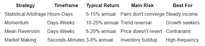
Comparing Strategies:
So, What Does This Mean For You?
If you want to step into quantitative trading, your first job isn’t to code a model—it's to ask a great question. That means defining your goal, time frame, constraints, and market conditions. The math comes after.
Quant strategies are simply targeted solutions to well-framed problems. The better your question, the more useful (and profitable) your model.
To start quantitative trading:
Pick one strategy—start with momentum, it's simplest.
Get historical price data for 10 stocks
Code the basic formula
Test it on paper for 3 months before using real money
The difference between potential and profit is action. Let your curiosity drive the research, your data guide the models, and your discipline seal the results.